This is the paper in full, written in San Diego and dated 3 February 2006. The text is as first published, corrected only for grammar, punctuation and figure numbering — no arguments have been added or removed.
1. The Cartesian Coordinate System
Before we can talk about verbogeometry, we must look at some pertinent elements of analytic geometry. Concerning this paper on verbogeometry, you should know enough analytic geometry to plot points and a few basic equations on a Cartesian coordinate system. However, I would like to believe that anyone should be able to enjoy some understanding of verbogeometry. If you need a refresher on the Cartesian coordinate system, you may want to look online; Wikipedia has a nice overview of the system.
When we look at the two-dimensional axes of a Cartesian coordinate system, we can see that by picking a point somewhere on the plane defined by those axes there is a relationship of that point back to the origin. This relationship is understood through the nomenclature of the coordinate pair (x, y), where x and y are distances along each axis from the origin. Furthermore, if we draw lines from a newly created point, perpendicular to both the x-axis and the y-axis, and take into consideration the axis system in the background, then we will make a rectangle (see Figure 1).
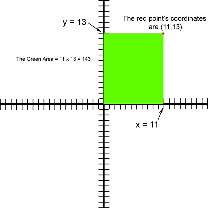
The area of a rectangle is the product of the lengths of its sides, and in the upcoming example the product of the values of the x- and y-coordinates of this point. Of course, this one is a special case because we used the axis origin as our starting point. Example: let us arbitrarily pick a point defined by the x-y coordinates (11, 13) and draw lines perpendicular to the axes to illuminate what I have just said. The area of any rectangle is equal to its height multiplied by its base (the product of the lengths of its sides). We have a green rectangle delineated on our axis system (see Figure 1). The height of our rectangle is 13 units and its base is 11 units. The area of our rectangle is 143 square units, or 13 × 11 = 143.
This latter example is one of pure mathematics. However, if we want to use mathematics as a language, then we will have to apply concepts, or words, to our axis system.
Let us look at a typical physics problem of distance, velocity, and time displayed on a two-dimensional axis system. Let us assign the y-axis to be levels of velocity in units of miles per hour and the x-axis to be amounts of time in units of hours (see Figure 2).
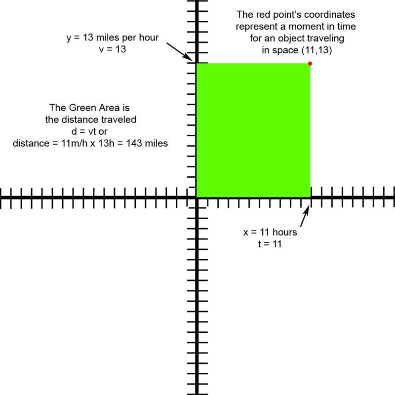
The distance of an object traveling in space is equal to the velocity of the object multiplied by the average time it is traveling in space, or d = vt. Let us use the same pure-mathematical example as before, but by contextualizing the axes and assigning the y-axis to represent velocity and the x-axis to represent time, our original point from the last example, (11, 13), has a new meaning. To reiterate: the point before was in the realm of pure mathematics, but now the point represents a moment in time of a speeding object. The object is traveling 13 miles per hour and has been traveling for 11 hours. So to calculate (d = vt) the distance the object has traveled, we must multiply the velocity by the time, or 13 miles per hour times 11 hours, which equals 143 miles.
In essence, what we have done has been to assign a concept, by using words (velocity and time), to our axis system. Moving our attention up or down on the y-axis displays different values of velocity. Moving left and right on the x-axis displays different amounts of duration, or time. Physical experimentation can easily verify the veracity of this equation. In addition, the same experimentation verifies the verbal concepts and their relationship to each other that we have assigned to our axis system. We can see the relationship between the concepts of distance, velocity, and time spread out on a two-dimensional plane via our axis system. It is important to note that these concepts occupy orthogonal spaces, as do the concepts in all equations of the form A = BC. Furthermore, the equation makes sense because it matches our perceptions of the event, and the axis system is a model of our experience. Although the use of the latter equations was for the purpose of denotation, verbogeometry is more interested in the use of equations for connotation and in witnessing dissimilar concepts forced into orthogonal spaces to create metaphor.
2. The Mechanics of Verbogeometry
2.1 Word-Axes and Word-Planes
One of the tenets of verbogeometry and mathematical poetry is that you “calculate” values of quality as if they were quantity. Of course this seems to be nonsense, but then one must realize that paradox is the mathematical structure of metaphor. When quality and quantity are synonymous, the mathematical equations automatically transcend the normal duty of denotation and enter into the realms of connotation. This concept also bears some relationship to the different concepts of infinity pioneered by the Russian-German mathematician Georg Cantor, namely the infinities in gradation relative to the infinities in counting.
Another tenet of verbogeometry is that it recognizes only a few varieties of antonym. A simple antonym is a word whose antonym is a direct negation (example: just / unjust, probable / improbable, or fertile / infertile). A complex antonym is a word whose antonym is not a direct negation (example: just / unfair, probable / doubtful, or fertile / barren). There are also gradable (gradient) antonyms, which are pairs that express relationships in a continuum, such as up and down. Complementary antonyms are pairs that express an either/or relationship, such as dead or alive. Verbogeometry uses all antonyms as if they were gradable. It is easy to find examples where poets use complementary antonyms as if they were gradable in order to create certain metaphors. Example: “Bob showed up half dead to work today.”
Within the boundaries of verbogeometry, it is important to understand that we view words as objects floating in space. When we focus on single words, with no context, they are inert and alone, relating to no other words. However, when we focus on words that have a synonymous partner, we can easily imagine a line in space between the words. Probable and improbable are good examples of simple antonyms that we can view as connected by a line (see Figure 3).
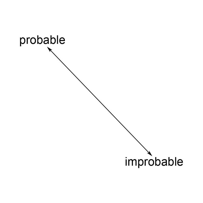
Life is full of dualities; it is hard to think about qualities without thinking about opposing ideas. We can view our probable / improbable one-dimensional line as a number line, but instead of values of numbers on the line, we think in terms of having different levels of meaning between the two words residing at each end of the line. Because a number line is a one-dimensional axis, it is easy to visualize a word-axis as an axis for a single spatial dimension. We call any pair of words connected by a line a word-axis. Two perpendicular number lines, or word-axes, make a two-dimensional word-axis as well as defining a word-plane. We also have the ability to view the word-plane as an infinite number of coordinates delineated by the word-pairs, much like the infinite number of coordinate pairs contained within a Cartesian coordinate system described in the realm of analytic geometry.
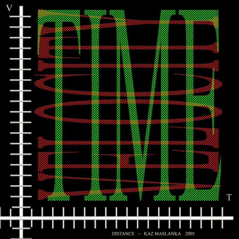
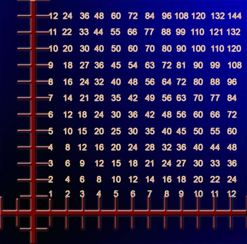
Figure 4 shows a visualization for the physics equation distance = velocity multiplied by time. Notice that the y-axis displays velocity and the x-axis displays time. When we multiply and blend the words in an infinitesimal weave, we arrive at the concept of distance in a tessellated product of the concepts of velocity and time. In other words, by positioning the two axes perpendicular to each other, we view every value on one word-axis in relation to every value on the other word-axis. This method affords us a way to “feel” the entire word-plane, or axis system, with all its different augmented values and gradations. When we multiply two word-axes together, we conceptually tessellate a two-dimensional plane with different semantic values of the two words blended and augmented. If we were to take a normal Cartesian coordinate system and multiply the positive x integers (1 through 12) by the positive y integers (1 through 12), we would get a tessellated plane as in Figure 5 (notice the intensity of blue relative to the value of the numbers).
To help us further visualize this concept, let us create a word-axis using the words red and green. In this instance, we are going to use red and green as nouns instead of adjectives (we will use colors as adjectives later). Let us multiply a red-green axis by another red-green axis and view it visually (see Figure 6). Multiplication of colors is similar to color addition, except that the disparate intensities of the colors are greater and follow a pattern similar to the one shown in Figure 5. The value of the “numbers” is subjective and not as important as the relationship between the “numbers.”
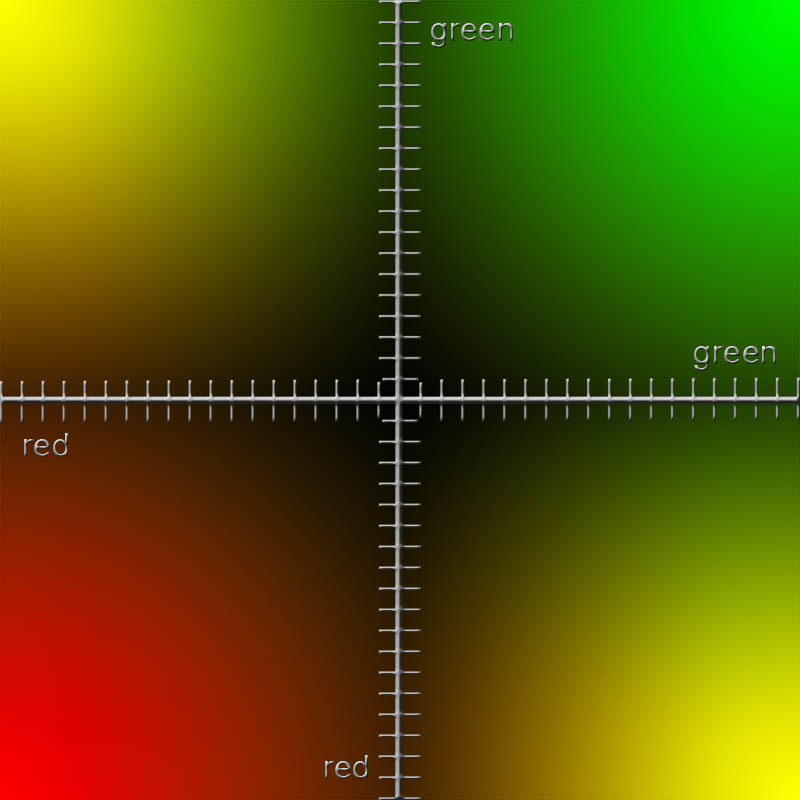
Figure 6 helps us to visualize different word meanings spread across a word-plane.
Let us create another example using two different word-axes. However, let us use two differently colored word-axes instead of both axes being the same colors, as in our previous example. Then let us break down what we have just accomplished and look at the axes separately. After that, we will superimpose a set of different word-axes upon our color axes to compare how the system works.
To facilitate visualizing two different word-axes, let us look at an example with the word-axes red-green and blue-orange multiplied by each other and mapped on a Cartesian coordinate system (see Figure 7).
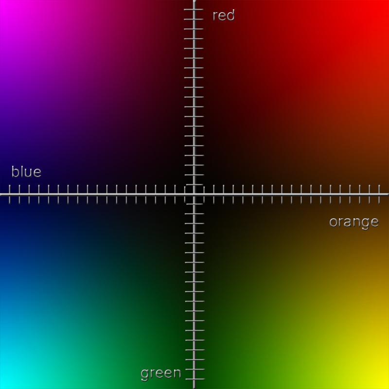
Figure 7 is composed of two axes: a red-green axis in the vertical and a blue-orange axis in the horizontal. Let us look at the red-green vertical axis separately (see Figure 8),
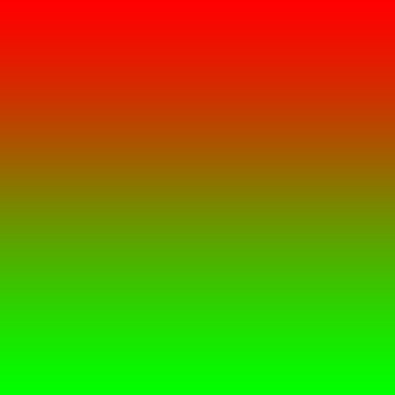
and, separately from Figure 7, the blue-orange horizontal axis as well (see Figure 9).
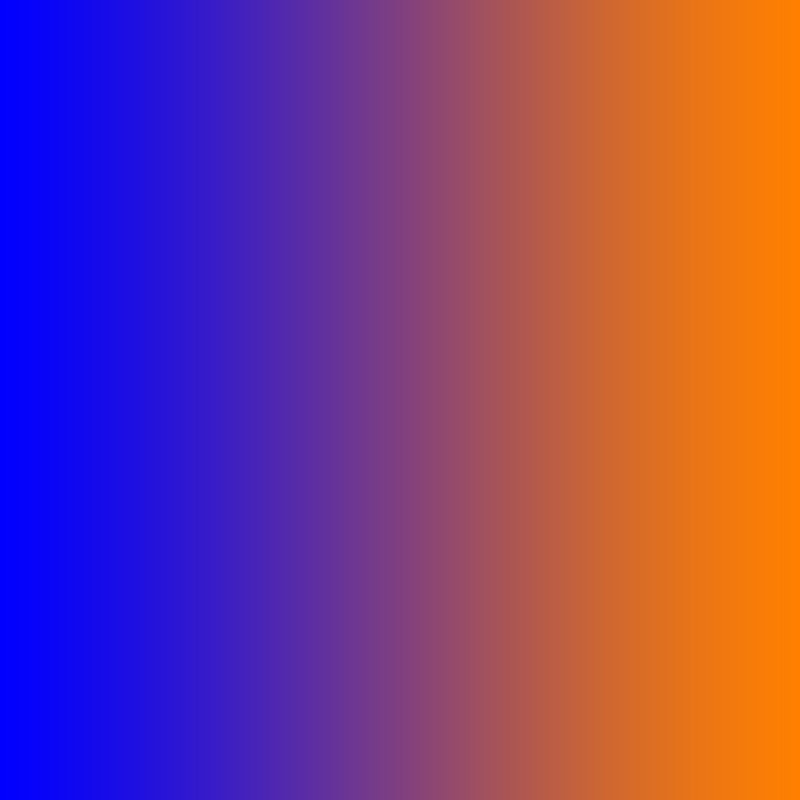
Furthermore, notice the direction of the gradations. When we place the axes perpendicular to each other and multiply them together, we see the color tessellations of the word-plane (see Figure 7).
What is nice about using colors for our examples is that words used for colors function as both nouns and adjectives, depending on our intent. When we map a word-plane with word-axes that comprise colors and we use them as adjective synonyms, then this word-plane serves as a paradigm, or a pedagogical tool, to serve as a general model for understanding all two-axis synonym word-planes. Example: let us create a word-plane using the two word-axes noble / ignoble and just / unjust (see Figure 10).
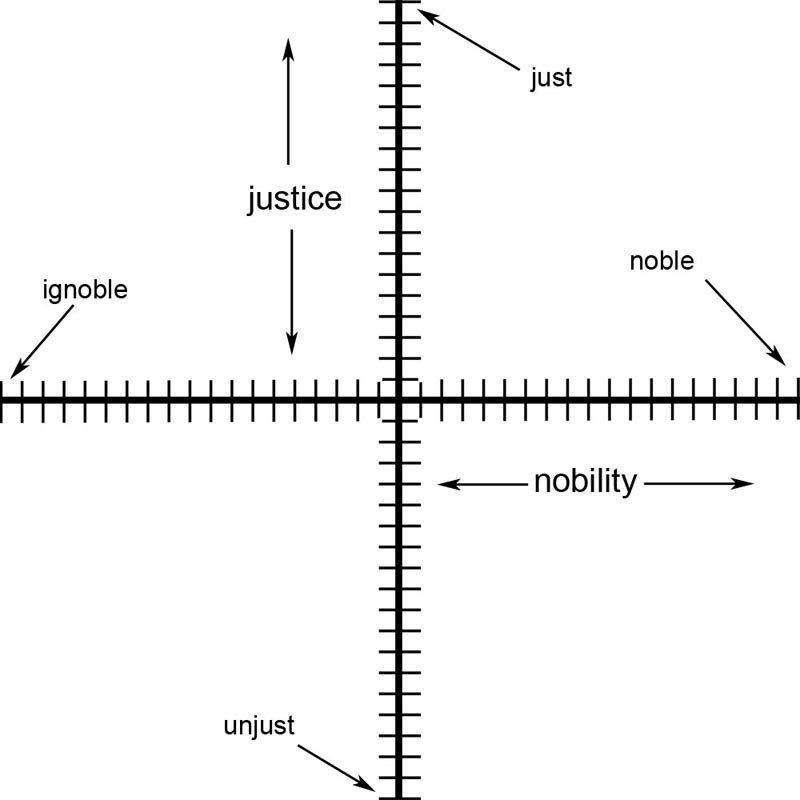
The next step would be to superimpose the noble / ignoble, just / unjust word-plane onto our previous word-plane of blue / orange, red / green. In essence, we are pretending the color blue means ignoble, orange means noble, red means just, and green means unjust. Now we can see the meanings blend into each other in the different areas of our word-plane (see Figure 11).
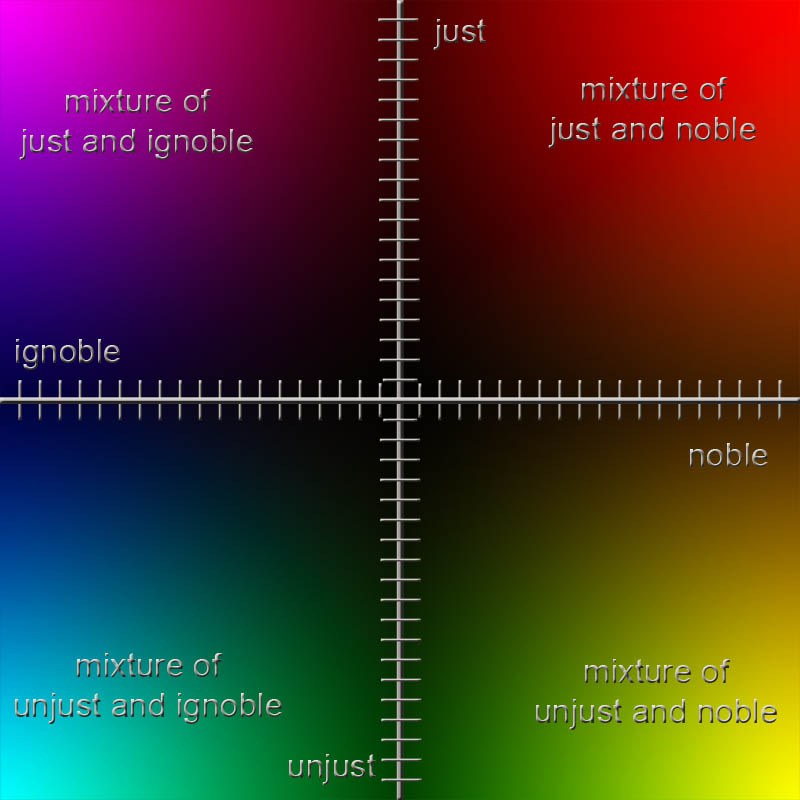
We can see the color purple as a blend of ignoble and just, red-orange as a blend of just and noble, yellow-green as a blend of noble and unjust, and blue-green as a blend of ignoble and unjust. For the record, I certainly am not trying to say there is a relationship of ignobility and injustice with the color blue-green. This example is just a tool to help us with our own concept of visualizing a word-plane. However, we could create a different, but in my opinion limited, set of color metaphors for noble / ignoble and just / unjust. Or we could look at our color example as adjectives on their own merit. This method would automatically help us see them as metaphors. Example: She was red hot. He had a blue day. He was so green he did not know what was happening. Multiplying adjective word-axes together instantly creates metaphors.
2.2 Word-Coordinate Pairs
We have witnessed a word-axis with different values of an antonym pair along a particular axis, x or y, in one dimension (see Figure 3). We have also seen a word-plane with values of two antonym pairs along two axes, x and y, in two dimensions (see Figure 10). Furthermore, we can have word-cubes along the x-, y-, and z-axes in the third dimension and word-hypercubes in the fourth dimension, or we can have antonymic pairs in innumerable dimensions. There is no limit to the dimensional palette for our expressions. Each antonym word-pair adds a new spatial dimension to our expressive construction.
Let us talk about the spatial accuracy in defining the location of words in space. Once again, let us look at Figure 10 and notice the antonym word-pairs just / unjust and noble / ignoble. However, let us focus our attention on the word-axis just / unjust. We know that we have defined a one-dimensional word-axis with different values of just and unjust, but we do not know exactly where each of the words is located along the axis. We have no quantitative value for just or unjust. However, we do have a qualitative value, and we know that the word exists somewhere on the axis. What is most important to us in verbogeometry is not the value as such, but the spatial relationship of the values to each other in space. Because the value, or the meaning, of a word is relative to the context in which it is used, each viewer individually creates his or her own context for meaning. Therefore, exact quantification of the word, or of its location in space, is not possible. However, in some cases it may be possible to restrict the context to a level where repeatable correlations exist, but those studies are more akin to denotation for the purpose of science. Scientific experimentation “proves” the equation to be mathematically correct and workable within a range of acceptability. In other words, experimental data defines the viability of the relationships between the concepts in a scientific equation. On a side note: when scientific equations are in the intuitive stages of development, there may be an argument to claim that they are in the realm of art; I personally might accept this view if it were not for the fact that their intention is not to make art. In verbogeometry, we construct equations based on relationships between the qualities of our experiences in order to evoke meaningful aesthetic expressions, of which most are connotative but some may be denotative.
Let us get back to the Cartesian coordinate system for a moment and reiterate the idea of coordinate pairs. A point on a two-dimensional coordinate system would have values for x and y and would be expressed as (x, y) (see Figure 1). A point on a three-dimensional axis system would have values for x, y, and z and would be expressed as (x, y, z). A four-dimensional point would be expressed as (x, y, z, w), a five-dimensional point as (x, y, z, w, v), and so on.
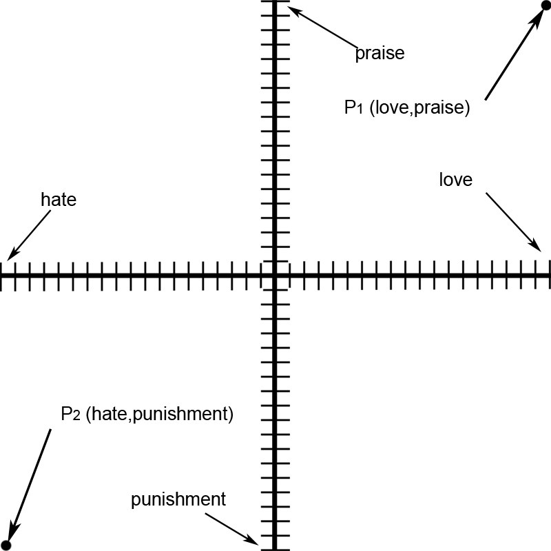
Before we get into multidimensional word-axes, let us just look at a simple two-dimensional word-plane with two word-axes (see Figure 12).
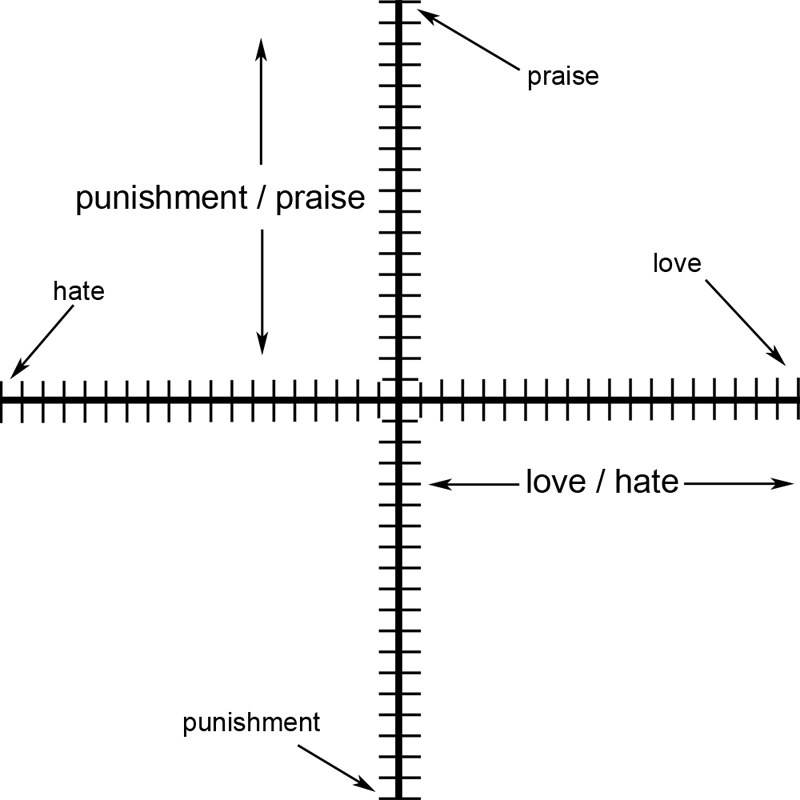
The vertical axis is a synonym word-pair of praise and punishment, and the horizontal axis is a synonym word-pair of love and hate. It is very important to realize that not only do the words love and hate define the identity of the horizontal, or x-, axis; they also hold conceptual points in space along the axis, and the same is true for praise and punishment with respect to the y-axis. The words, which are conceptual points in space, define a metaphoric value along their respective axes and can be notated as a coordinate pair similar to (x, y). So you may ask, what would a coordinate word-pair look like? Let us look at the two points identified as point 1, or P1(love, praise), and point 2, P2(hate, punishment) (see Figure 13).
2.3 The Midpoint Formula in Verbogeometry
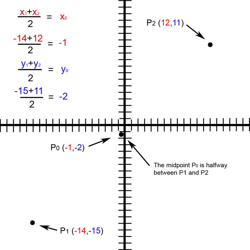
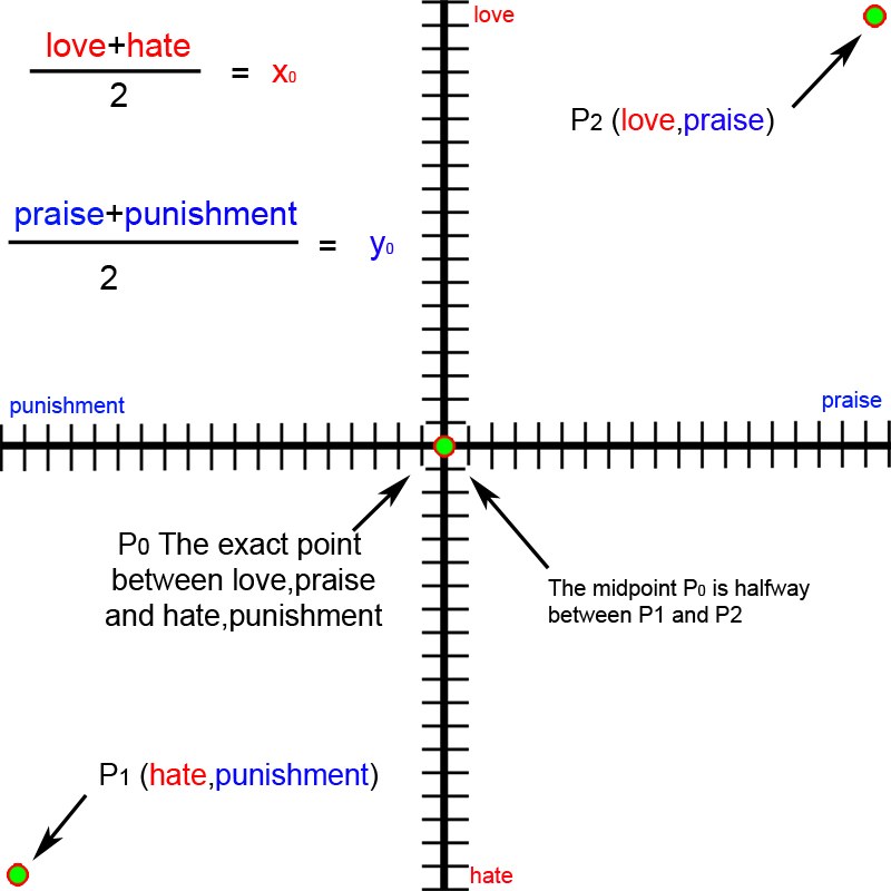
Any analytic geometry equation can use coordinate word-pairs instead of numbers to express poetic forms. Let us use the midpoint formula to express the exact point between the two points P1(love, praise) and P2(hate, punishment) from Figure 13. Before we look at coordinate word-pairs, let us refresh the use of the midpoint formula in analytic geometry. To find the midpoint between two points on a Cartesian coordinate system, we add the x-coordinates together and divide by 2 to find the x-value for the midpoint, and we also add the y-coordinates together and divide by 2 to find the y-value for the midpoint, or (x1 + x2)/2 = x0 and (y1 + y2)/2 = y0.
Let us look at an example of finding the midpoint P0 between the points P1(−14, −15) and P2(12, 11) utilizing the midpoint formula. x1 = −14 and x2 = 12, so substituting our numbers into the variables of the equation (x1 + x2)/2 = x0, we get (−14 + 12)/2 = −1. Also, y1 = −15 and y2 = 11, so substituting our numbers into the variables of the equation (y1 + y2)/2 = y0, we get (−15 + 11)/2 = −2. Therefore P0 = (−1, −2) (see Figure 14).
Let us now take a different approach and replace the numeric variables in the midpoint equation with the words/concepts love, hate, praise, and punishment. We will use the form of coordinate word-pairs P1(love, praise) and P2(hate, punishment). The midpoint formula now shows us that P0(x0, y0) will be formed by the substitution of (x1 + x2)/2 = x0 with (love + hate)/2 = x0, and of (y1 + y2)/2 = y0 with (praise + punishment)/2 = y0. Now we have expressed the exact point between love, praise and hate, punishment (see Figure 15).
2.4 Verbogeometry with Trigonometry
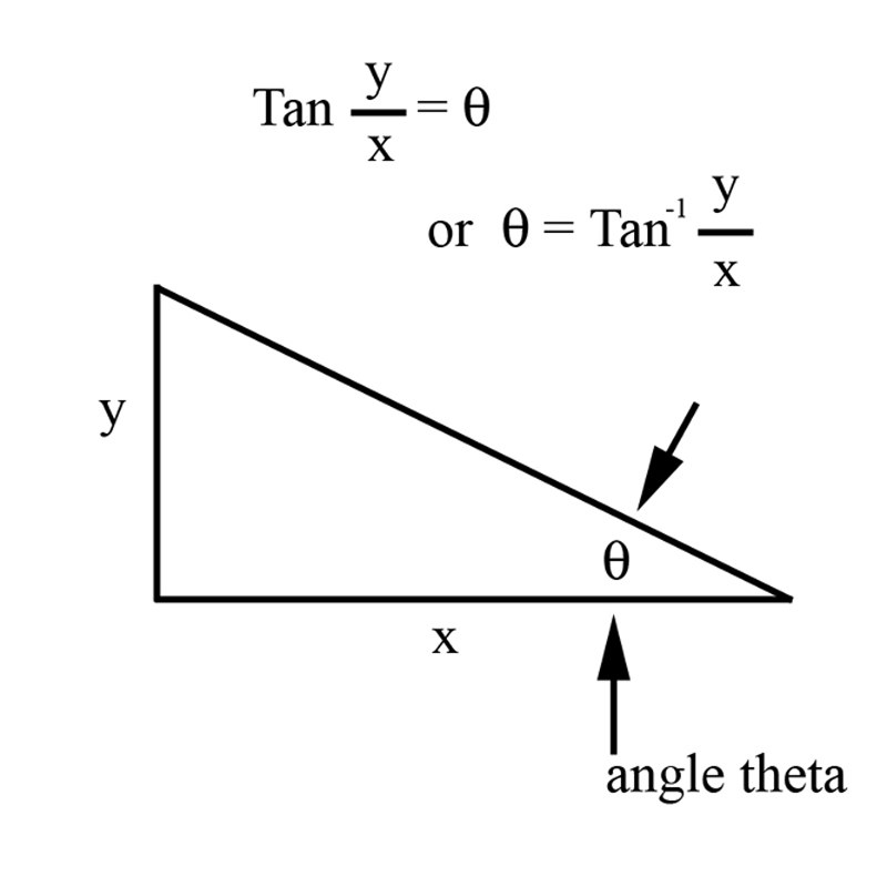
First, let us solve a pertinent traditional trigonometric problem, which requires a solution for an angle. Let us make theta the variable of the angle in question. The tangent of an angle in a right triangle is defined as the ratio of the side opposite the angle theta to the side adjacent to the angle theta. If we call the side opposite distance “y” and the side adjacent distance “x,” we then arrive at tan(theta) = y/x (see Figure 16).
It also follows that if we know the lengths of two sides of a right triangle, we can find all the angles. Let us look at an example with the side opposite angle theta being 3 and the side adjacent to angle theta being 4. Let us now solve for the angle theta. We know that y/x = tan(theta), so it follows that 3/4 = tan(theta). To uncover the value of theta, we must take the inverse tangent of 3/4. Symbolically, this is stated as “theta = inverse tan(y/x),” or approximately 36.87 degrees (see Figure 17).
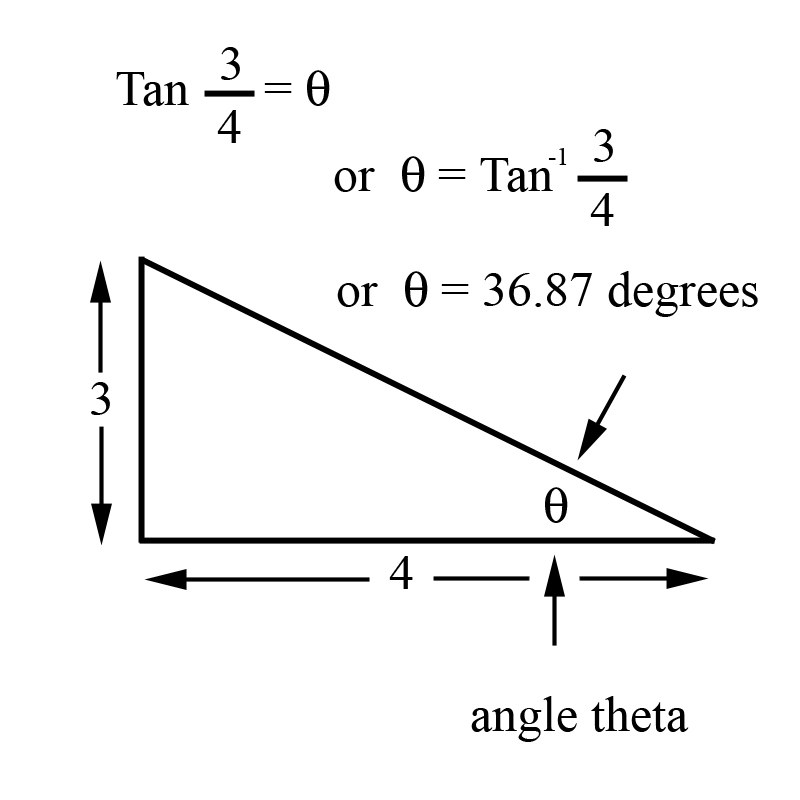
In general, to reveal the angle after you have calculated the value for the tangent y/x, your choice is to find the angle in a trigonometric table (the old method) or to plug the values into a handheld calculator.
Now let us look at a similar expression using verbogeometry and looking for the value of angle theta. This time we define the y distance as the difference between the concepts of barren and infertile (think number line again), and let us define the x distance as the difference between the concepts of infertile and fertile (see Figure 18).
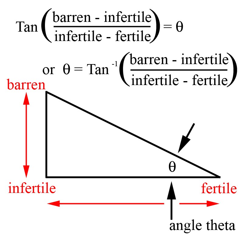
If we want to know the angle theta, we have to take the inverse tangent of y/x, or the inverse tangent of (barren − infertile)/(fertile − infertile) (see Figure 18).
2.5 Prismatic Structures in Verbogeometry
Notice that “barren and fertile” is a complex antonym pair and “fertile and infertile” is a simple antonym pair, as previously defined.
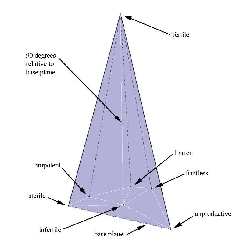
This is interesting because we can see that there exists in verbogeometry a geometric construction where a line expressed as a simple antonym is normal (90 degrees) to a plane containing all of the complex antonyms related to the line which is expressing the simple antonym.
To illustrate this idea, let us look again at the relationship between the simple antonyms “fertile” and “infertile” and the synonyms “barren,” “fruitless,” “unproductive,” “sterile,” and “impotent,” which reside on the plane that is normal (90 degrees) to the line created by the simple antonyms. Furthermore, you can draw lines from all of the synonyms back to the complex antonym “fertile” (see Figure 19).
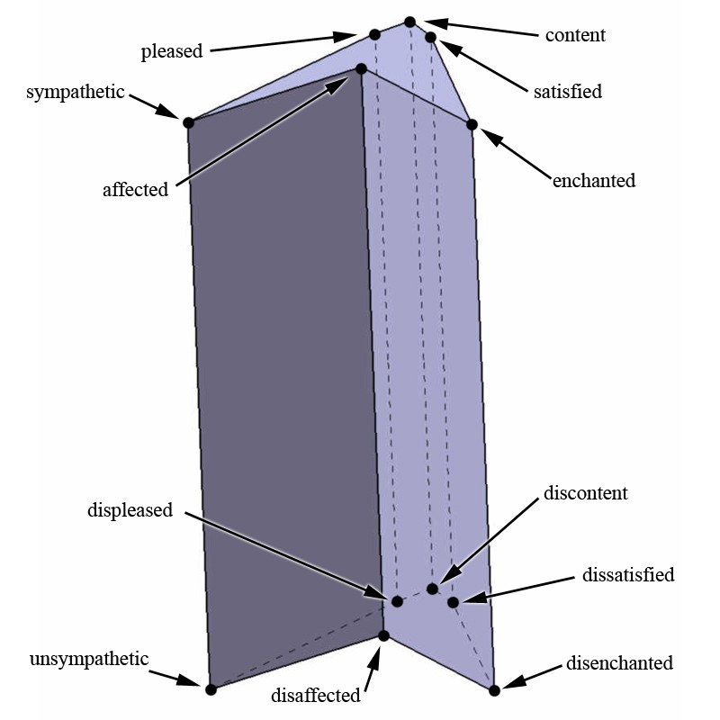
This idea also lends itself to prismatic structures where we have a group of parallel simple antonyms whose endpoints construct polygonal faces on two parallel synonym-planes (see Figure 20). Example: let us define one synonym-plane containing the words “pleased,” “content,” “affected,” “satisfied,” “enchanted,” and “sympathetic.” The other plane contains the following simple antonyms for the previous group of synonyms: “displeased,” “discontent,” “disaffected,” “dissatisfied,” “disenchanted,” and “unsympathetic.” Because the synonyms of one plane have corresponding simple antonyms which create lines 90 degrees from the synonym-plane, the simple antonyms are synonyms of each other and reside on their own individual synonym-plane; and because the lines are 90 degrees to each other, the planes must be parallel. The former verbiage is a lot easier to understand visually (see Figure 20).
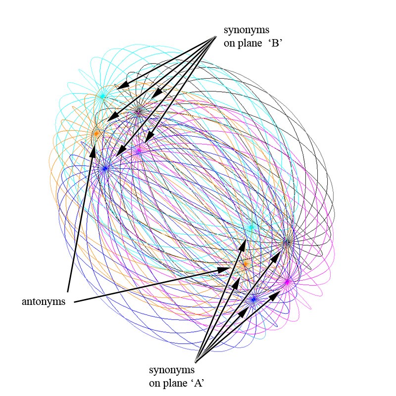
On a side note: everything that we have been talking about up to this point has been viewed in Euclidean space. Not much time has been spent exploring verbogeometry outside of Euclidean space. However, I see that there can be a lot more thought devoted to evolving models of verbogeometry in other spaces. For example, instead of viewing antonyms and all the varying meanings spread out across a number line, we may think of the antonyms as magnetic dipoles. Furthermore, all the varying meaning between them is analogous to a magnetic flux. Yet again, another view may be looking at the antonyms residing at the endpoints of a major axis of a three-dimensional ellipsoid, with the varying meanings residing on the surface of the ellipsoid (see Figure 21).
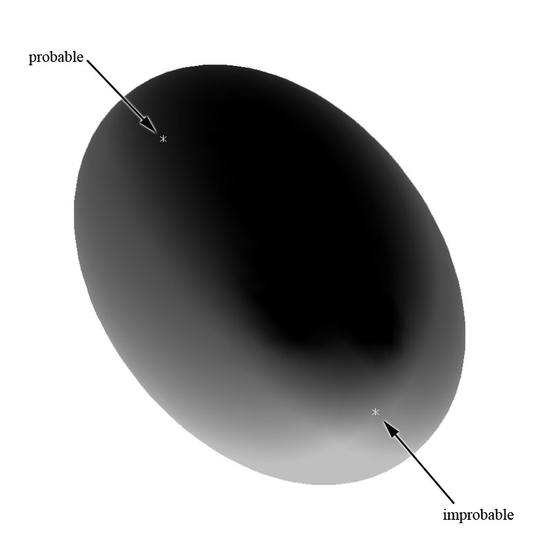
Figure 22 shows an ellipsoidal, flux-like paradigm for the previous prismatic structure (see Figure 20).
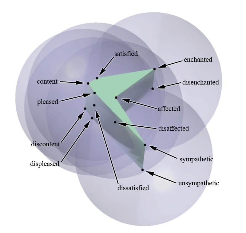
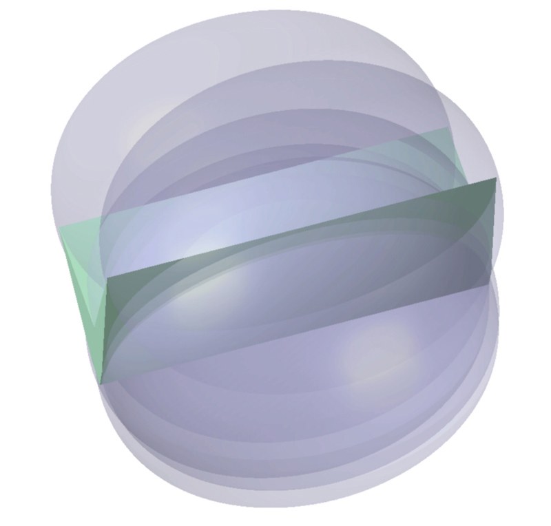
Figure 23 shows an unlabeled side view.
It may be easier to see the ellipse structure if it is shown as a wireframe (see Figure 24).
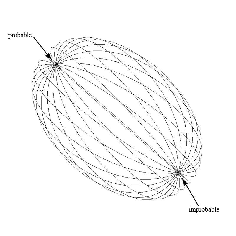
Figure 25 shows five parallel word-axes in a wireframe structure.
2.6 The Distance Formula and the Pythagorean Theorem
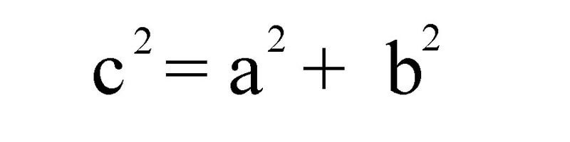
The distance formula uses the Pythagorean theorem to calculate distances on the Cartesian coordinate system. The Pythagorean theorem says that the square of the hypotenuse of a right triangle is equal to the sum of the squares of its sides (see Figure 26).
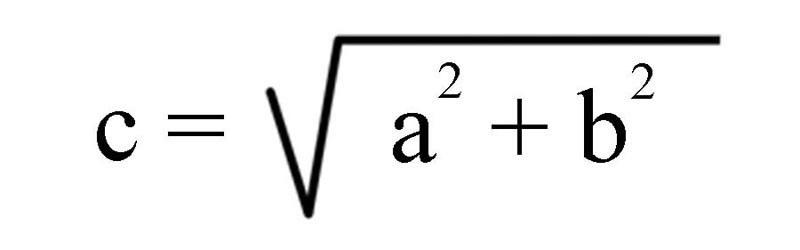
Solving for c, we get the following (see Figure 27).
Let us plot two points on a two-dimensional axis system, P1(9, 10) and P2(4, 3). If we draw a line between the points, and lines parallel to the axes, we can obtain a right triangle (see Figure 28).
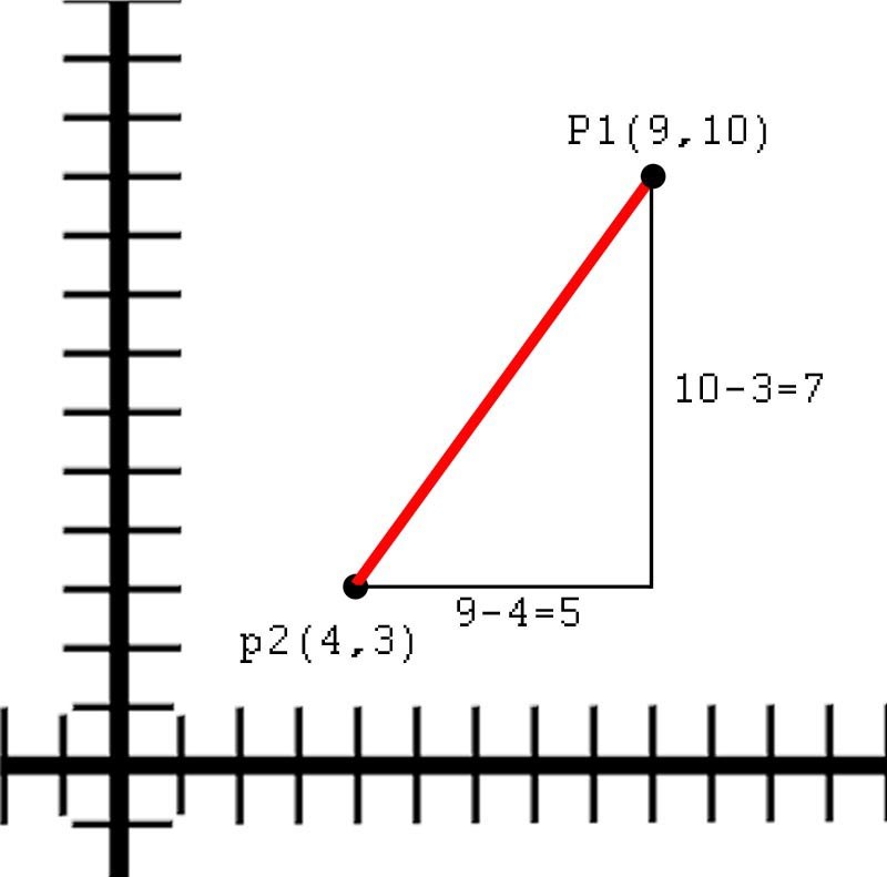
To solve for the length of the hypotenuse, we first find the difference between the x-values and the y-values to create the sides of the triangle, then we plug the values into the Pythagorean theorem. The x-value is 9 − 4 = 5, and the y-value is 10 − 3 = 7. Now we plug it into the equation and we get the expression in Figure 29.
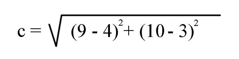
The distance, or length, of the hypotenuse would be the square root of 74, or approximately 8.602.
The distance formula is thus, given two points (x1, y1) and (x2, y2) (see Figure 30):
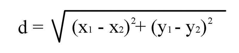
Now, what we have been looking at up till now has been in two dimensions, but we can also express a distance in many dimensions. Let us look at two points in three dimensions: P1(x1, y1, z1) and P2(x2, y2, z2). If we were to put these two points into the distance formula, it would look like what is shown in Figure 31.

It is evident that we can use the distance formula in uncountable dimensions; all we have to do is add another dimensional term to the formula for every dimension we wish to express.
2.7 The Distance Formula and Verbogeometry
As we have seen, to calculate the distance between two points we need to describe our points by their coordinates, using the nomenclature of the coordinate pair. Let me reiterate: describing a point in verbogeometry is no different from using numerical coordinates, except that we use words. Let us look again at the example in Figure 15, where we used the midpoint formula to find the exact point between the points P1(love, praise) and P2(hate, punishment); but instead of putting them into the midpoint formula, let us put them into the distance formula (see Figure 32).
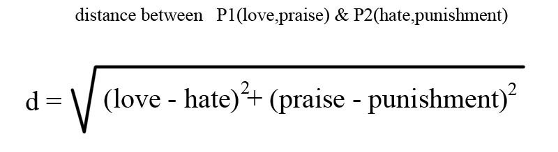
Here we have an expression for the distance between the points P1(love, praise) and P2(hate, punishment) in two dimensions. But we can also use verbogeometry in any number of dimensions, including hyper-dimensions. Before we look at hyper-dimensional verbogeometry, let us look at another example, which we will express in the third dimension. The following example uses a three-dimensional Cartesian coordinate system with three simple antonym word-axes (see Figure 33). The first axis is noble / ignoble, the second axis is just / unjust, and the third axis is loyal / disloyal.
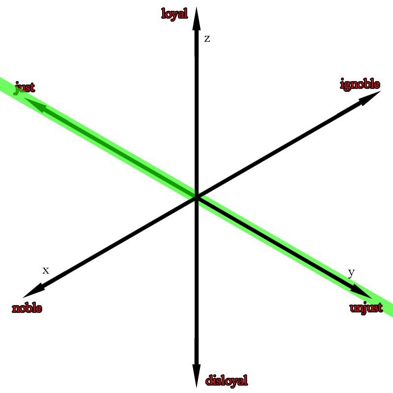
Now let us look at the expression for the distance between the points P1(noble, just, loyal) and P2(ignoble, unjust, disloyal) (see Figure 34).
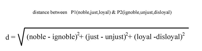
Notice that the green line in Figure 33 is the visual representation of the mathematical expression above. However, it would be much easier to visualize if we were able to rotate the axes. Figure 33 is an isometric view, which I chose to use because it is best for viewing the axes, but unfortunately at the expense of viewing the spatial orientation of the green line.
Now let us look at verbogeometry in a hyper-dimension. Let us look at the distance formula used in seven dimensions.
Figure 35 shows the mathematical poem “A God Path” (1 + 1 + 1 + 1 + 1 + 1 + 1 = 1). This is a metaphorical piece that creates a metaphoric path from the concept of confusion to the point where seven deities meet. The piece uses the analytic geometry distance formula in a seven-dimensional space where each dimension is a gradation from confusion to a point where a deity exists.
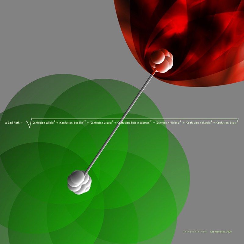

Let us look at the coordinate pairs for these two points: P1(confusion, confusion, confusion, confusion, confusion, confusion, confusion) and P2(Allah, Buddha, Jesus, Spider Woman, Vishnu, Yahweh, Zeus).
3. Conclusion
What I have shown here scratches the surface of the possibilities of verbogeometry. Verbogeometry can be taken in vast directions that I have not covered and will not be able to cover. I hope that in the future more people will join in to explore the possibilities of verbogeometry.
Reference
- “Cartesian coordinate system.” Wikipedia. http://en.wikipedia.org/wiki/Cartesian_coordinate_system
Verbogeometry poems
- The Exact Point Between Love, Hate, Praise and Punishment 2000
- A God Path 2000
- The Virtuous Sphere 2000
- Theta 2002
- Centered 2005
- The Transformation of Poison 2006
- The Muses 2014